histogram

Histogram plot

expand all in page

Description

Histograms are a type of bar plot for numeric data that group the data into bins. After you create aHistogramobject, you can modify aspects of the histogram by changing its property values. This is particularly useful for quickly modifying the properties of the bins or changing the display.

Creation

Syntax

histogram(X)

histogram(X,nbins)

histogram(X,edges)

histogram('BinEdges',edges,'BinCounts',counts)

histogram(C)

histogram(C,Categories)

histogram('Categories',Categories,'BinCounts',counts)

histogram(___,Name,Value)

histogram(ax,___)

h = histogram(___)

Description

example

histogram(X)creates a histogram plot ofX. Thehistogramfunction uses an automatic binning algorithm that returns bins with a uniform width, chosen to cover the range of elements inXand reveal the underlying shape of the distribution.histogramdisplays the bins as rectangles such that the height of each rectangle indicates the number of elements in the bin.

example

histogram(X,nbins)uses a number of bins specified by the scalar,nbins.

example

histogram(X,edges)sortsXinto bins with the bin edges specified by the vector,edges. Each bin includes the left edge, but does not include the right edge, except for the last bin which includes both edges.

histogram('BinEdges',edges,'BinCounts',counts)manually specifies bin edges and associated bin counts.histogramplots the specified bin counts and does not do any data binning.

example

histogram(C), whereCis a categorical array, plots a histogram with a bar for each category inC.

histogram(C,Categories)plots only the subset of categories specified byCategories.

histogram('Categories',Categories,'BinCounts',counts)manually specifies categories and associated bin counts.histogramplots the specified bin counts and does not do any data binning.

example

histogram(___,Name,Value)specifies additional options with one or moreName,Valuepair arguments using any of the previous syntaxes. For example, you can specify'BinWidth'and a scalar to adjust the width of the bins, or'Normalization'with a valid option ('count','probability','countdensity','pdf','cumcount', or'cdf')使用不同类型的正常化。对于一个list of properties, seeHistogram Properties.

histogram(ax,___)plots into the axes specified byaxinstead of into the current axes (gca). The optionaxcan precede any of the input argument combinations in the previous syntaxes.

example

h= histogram(___)返回一个Histogramobject. Use this to inspect and adjust the properties of the histogram. For a list of properties, seeHistogram Properties.

Input Arguments

expand all

`X`—数据分发垃圾箱中
vector|matrix|multidimensional array

数据分发垃圾箱中, specified as a vector, matrix, or multidimensional array. IfXis not a vector, thenhistogramtreats it as a single column vector,X(:), and plots a single histogram.

histogramignores allNaNandNaTvalues. Similarly,histogramignoresInfand-Infvalues, unless the bin edges explicitly specifyInfor-Infas a bin edge. AlthoughNaN,NaT,Inf, and-Infvalues are typically not plotted, they are still included in normalization calculations that include the total number of data elements, such as'probability'.

Note

IfXcontains integers of typeint64oruint64that are larger thanflintmax, then it is recommended that you explicitly specify the histogram bin edges.histogramautomatically bins the input data using double precision, which lacks integer precision for numbers greater thanflintmax.

`C`—Categorical data
categorical array

Categorical data, specified as a categorical array.histogramdoes not plot undefined categorical values. However, undefined categorical values are still included in normalization calculations that include the total number of data elements, such as'probability'.

Data Types:categorical

`nbins`—Number of bins
positive integer

Number of bins, specified as a positive integer. If you do not specifynbins, thenhistogramautomatically calculates how many bins to use based on the values inX.

Example:histogram(X,15)creates a histogram with 15 bins.

`edges`—Bin edges
vector

Bin edges, specified as a vector.edges(1)is the left edge of the first bin, andedges(end)is the right edge of the last bin.

The valueX(i)is in thekth bin ifedges(k)≤X(i)<edges(k+1). The last bin also includes the right bin edge, so that it containsX(i)ifedges(end-1)≤X(i)≤edges(end).

For datetime and duration data,edges必须是一个datetime或持续时间向量在单调吗ally increasing order.

`Categories`—Categories included in histogram
cell array of character vectors|categorical array|string array

Note

This option only applies to categorical histograms.

Categories included in histogram, specified as a cell array of character vectors, categorical array, or string array.

If you specify an input categorical arrayC, then by default,histogramplots a bar for each category inC. In that case, useCategoriesto specify a unique subset of the categories instead.
If you specify bin counts, thenCategoriesspecifies the associated category names for the histogram.

Example:h = histogram(C,{'Large','Small'})plots only the categorical data in the categories'Large'and'Small'.

Example:histogram('Categories',{'Yes','No','Maybe'},'BinCounts',[22 18 3])plots a histogram that has three categories with the associated bin counts.

Example:h.Categoriesqueries the categories that are in histogram objecth.

Data Types:cell|categorical|string

`counts`—Bin counts
vector

Bin counts, specified as a vector. Use this input to pass bin counts tohistogramwhen the bin counts calculation is performed separately and you do not wanthistogramto do any data binning.

The length ofcountsmust be equal to the number of bins.

For numeric histograms, the number of bins islength(edges)-1.
For categorical histograms, the number of bins is equal to the number of categories.

Example:histogram('BinEdges',-2:2,'BinCounts',[5 8 15 9])

Example:histogram('Categories',{'Yes','No','Maybe'},'BinCounts',[22 18 3])

`ax`—Target axes
`Axes`object|`PolarAxes`object

Target axes, specified as anAxesobject or aPolarAxesobject. If you do not specify the axes and if the current axes are Cartesian axes, then thehistogramfunction uses the current axes (gca). To plot into polar axes, specify thePolarAxesobject as the first input argument or use thepolarhistogramfunction.

Name-Value Arguments

Specify optional pairs of arguments asName1=Value1,...,NameN=ValueN, whereNameis the argument name andValueis the corresponding value. Name-value arguments must appear after other arguments, but the order of the pairs does not matter.

Before R2021a, use commas to separate each name and value, and encloseNamein quotes.

Example:histogram(X,'BinWidth',5)

The histogram properties listed here are only a subset. For a complete list, seeHistogram Properties.

`BarWidth`—Relative width of categorical bars
`0.9`(default) |scalar in range`[0,1]`

Note

This option only applies to histograms of categorical data.

Relative width of categorical bars, specified as a scalar value in the range[0,1]. Use this property to control the separation of categorical bars within the histogram. The default value is0.9, which means that the bar width is 90% of the space from the previous bar to the next bar, with 5% of that space on each side.

If you set this property to1, then adjacent bars touch.

Example:0.5

`BinLimits`—Bin limits
two-element vector

Bin limits, specified as a two-element vector,[bmin,bmax]. This option plots a histogram using the values in the input array,X,介于bminandbmaxinclusive. That is,X(X>=bmin & X<=bmax).

This option does not apply to histograms of categorical data.

Example:histogram(X,'BinLimits',[1,10])plots a histogram using only the values inXthat are between1and10inclusive.

`BinLimitsMode`—Selection mode for bin limits
`'auto'`(default) |`'manual'`

Selection mode for bin limits, specified as'auto'or'manual'. The default value is'auto', so that the bin limits automatically adjust to the data.

If you explicitly specify eitherBinLimitsorBinEdges, thenBinLimitsModeis automatically set to'manual'. In that case, specifyBinLimitsModeas'auto'to rescale the bin limits to the data.

This option does not apply to histograms of categorical data.

`BinMethod`—Binning algorithm
`'auto'`(default) |`'scott'`|`'fd'`|`'integers'`|`'sturges'`|`'sqrt'`| ...

Binning algorithm, specified as one of the values in this table.

Value	Description
`'auto'`	The default`'auto'`algorithm chooses a bin width to cover the data range and reveal the shape of the underlying distribution.
`'scott'`	Scott’s rule is optimal if the data is close to being normally distributed. This rule is appropriate for most other distributions, as well. It uses a bin width of`3.5std(X(:))numel(X)^(-1/3)`.
`'fd'`	The Freedman-Diaconis rule is less sensitive to outliers in the data, and might be more suitable for data with heavy-tailed distributions. It uses a bin width of`2IQR(X(:))numel(X)^(-1/3)`, where`IQR`is the interquartile range of`X`.
`'integers'`	The integer rule is useful with integer data, as it creates a bin for each integer. It uses a bin width of 1 and places bin edges halfway between integers. To avoid accidentally creating too many bins, you can use this rule to create a limit of 65536 bins (2¹⁶). If the data range is greater than 65536, then the integer rule uses wider bins instead. Note `'integers'`does not support datetime or duration data.
`'sturges'`	Sturges’ rule is popular due to its simplicity. It chooses the number of bins to be`ceil(1 + log2(numel(X)))`.
`'sqrt'`	The Square Root rule is widely used in other software packages. It chooses the number of bins to be`ceil(sqrt(numel(X)))`.

histogram并不总是选择使用th垃圾箱的数量ese exact formulas. Sometimes the number of bins is adjusted slightly so that the bin edges fall on "nice" numbers.

For datetime data, the bin method can be one of these units of time:

`'second'`	`'month'`
`'minute'`	`'quarter'`
`'hour'`	`'year'`
`'day'`	`'decade'`
`'week'`	`'century'`

For duration data, the bin method can be one of these units of time:

`'second'`	`'day'`
`'minute'`	`'year'`
`'hour'`

If you specifyBinMethodwith datetime or duration data, thenhistogramcan use a maximum of 65,536 bins (or 2¹⁶). If the specified bin duration requires more bins, thenhistogramuses a larger bin width corresponding to the maximum number of bins.

This option does not apply to histograms of categorical data.

Note

If you set theBinLimits,NumBins,BinEdges, orBinWidthproperty, then theBinMethodproperty is set to'manual'.

Example:histogram(X,'BinMethod','integers')creates a histogram with the bins centered on integers.

`BinWidth`—Width of bins
scalar

Width of bins, specified as a scalar. When you specifyBinWidth, thenhistogramcan use a maximum of 65,536 bins (or2¹⁶). If instead the specified bin width requires more bins, thenhistogramuses a larger bin width corresponding to the maximum number of bins.

For datetime and duration data, the value of'BinWidth'can be a scalar duration or calendar duration.

This option does not apply to histograms of categorical data.

Example:histogram(X,'BinWidth',5)uses bins with a width of 5.

`DisplayOrder`—Category display order
`'data'`(default) |`'ascend'`|`'descend'`

Category display order, specified as'ascend','descend', or'data'. With'ascend'or'descend', the histogram displays with increasing or decreasing bar heights. The default'data'value uses the category order in the input data,C.

This option only works with categorical data.

`DisplayStyle`—Histogram display style
`'bar'`(default) |`'stairs'`

Histogram display style, specified as either'bar'or'stairs'. Specify'stairs'to display a stairstep plot, which displays the outline of the histogram without filling the interior.

The default value of'bar'displays a histogram bar plot.

Example:histogram(X,'DisplayStyle','stairs')plots the outline of the histogram.

`EdgeAlpha`—Transparency of histogram bar edges
`1`(default) |scalar value between`0`and`1`inclusive

Transparency of histogram bar edges, specified as a scalar value between0and1inclusive. A value of1means fully opaque and0means completely transparent (invisible).

Example:histogram(X,'EdgeAlpha',0.5)creates a histogram plot with semi-transparent bar edges.

`EdgeColor`—Histogram edge color
`[0 0 0]`或黑色(default) |`'none'`|`'auto'`|RGB triplet|hexadecimal color code|color name

Histogram edge color, specified as one of these values:

'none'— Edges are not drawn.
'auto'— Color of each edge is chosen automatically.

RGB triplet, hexadecimal color code, or color name — Edges use the specified color.

RGB triplets and hexadecimal color codes are useful for specifying custom colors.

An RGB triplet is a three-element row vector whose elements specify the intensities of the red, green, and blue components of the color. The intensities must be in the range[0,1]; for example,[0.4 0.6 0.7].
A hexadecimal color code is a character vector or a string scalar that starts with a hash symbol (#) followed by three or six hexadecimal digits, which can range from0toF. The values are not case sensitive. Thus, the color codes'#FF8800','#ff8800','#F80', and'#f80'are equivalent.

Alternatively, you can specify some common colors by name. This table lists the named color options, the equivalent RGB triplets, and hexadecimal color codes.

Color Name	Short Name	RGB Triplet	Hexadecimal Color Code
`'red'`	`'r'`	`[1 0 0]`	`'#FF0000'`
`'green'`	`'g'`	`[0 1 0]`	`'#00FF00'`
`'blue'`	`'b'`	`[0 0 1]`	`'#0000FF'`
`'cyan'`	`'c'`	`[0 1 1]`	`'#00FFFF'`
`'magenta'`	`'m'`	`[1 0 1]`	`'#FF00FF'`
`'yellow'`	`'y'`	`[1 1 0]`	`'#FFFF00'`
`'black'`	`'k'`	`[0 0 0]`	`'#000000'`
`'white'`	`'w'`	`[1 1 1]`	`'#FFFFFF'`

Here are the RGB triplets and hexadecimal color codes for the default colors MATLAB^®uses in many types of plots.

RGB Triplet	Hexadecimal Color Code	Appearance
`[0 0.4470 0.7410]`	`'#0072BD'`
`[0.8500 0.3250 0.0980]`	`'#D95319'`
`[0.9290 0.6940 0.1250]`	`'#EDB120'`
`[0.4940 0.1840 0.5560]`	`'#7E2F8E'`
`[0.4660 0.6740 0.1880]`	`'#77AC30'`
`[0.3010 0.7450 0.9330]`	`'#4DBEEE'`
`[0.6350 0.0780 0.1840]`	`'#A2142F'`

Example:histogram(X,'EdgeColor','r')creates a histogram plot with red bar edges.

`FaceAlpha`—Transparency of histogram bars
`0.6`(default) |scalar value between`0`and`1`inclusive

Transparency of histogram bars, specified as a scalar value between0and1inclusive.histogramuses the same transparency for all the bars of the histogram. A value of1means fully opaque and0means completely transparent (invisible).

Example:histogram(X,'FaceAlpha',1)creates a histogram plot with fully opaque bars.

`FaceColor`—Histogram bar color
`'auto'`(default) |`'none'`|RGB triplet|hexadecimal color code|color name

Histogram bar color, specified as one of these values:

'none'— Bars are not filled.
'auto'— Histogram bar color is chosen automatically (default).

RGB triplet, hexadecimal color code, or color name — Bars are filled with the specified color.

RGB triplets and hexadecimal color codes are useful for specifying custom colors.

An RGB triplet is a three-element row vector whose elements specify the intensities of the red, green, and blue components of the color. The intensities must be in the range[0,1]; for example,[0.4 0.6 0.7].
A hexadecimal color code is a character vector or a string scalar that starts with a hash symbol (#) followed by three or six hexadecimal digits, which can range from0toF. The values are not case sensitive. Thus, the color codes'#FF8800','#ff8800','#F80', and'#f80'are equivalent.

Alternatively, you can specify some common colors by name. This table lists the named color options, the equivalent RGB triplets, and hexadecimal color codes.

Color Name	Short Name	RGB Triplet	Hexadecimal Color Code
`'red'`	`'r'`	`[1 0 0]`	`'#FF0000'`
`'green'`	`'g'`	`[0 1 0]`	`'#00FF00'`
`'blue'`	`'b'`	`[0 0 1]`	`'#0000FF'`
`'cyan'`	`'c'`	`[0 1 1]`	`'#00FFFF'`
`'magenta'`	`'m'`	`[1 0 1]`	`'#FF00FF'`
`'yellow'`	`'y'`	`[1 1 0]`	`'#FFFF00'`
`'black'`	`'k'`	`[0 0 0]`	`'#000000'`
`'white'`	`'w'`	`[1 1 1]`	`'#FFFFFF'`

Here are the RGB triplets and hexadecimal color codes for the default colors MATLAB uses in many types of plots.

RGB Triplet	Hexadecimal Color Code	Appearance
`[0 0.4470 0.7410]`	`'#0072BD'`
`[0.8500 0.3250 0.0980]`	`'#D95319'`
`[0.9290 0.6940 0.1250]`	`'#EDB120'`
`[0.4940 0.1840 0.5560]`	`'#7E2F8E'`
`[0.4660 0.6740 0.1880]`	`'#77AC30'`
`[0.3010 0.7450 0.9330]`	`'#4DBEEE'`
`[0.6350 0.0780 0.1840]`	`'#A2142F'`

If you specifyDisplayStyleas'stairs', thenhistogramdoes not use theFaceColorproperty.

Example:histogram(X,'FaceColor','g')creates a histogram plot with green bars.

`LineStyle`—Line style
`“- - -”`(default) |`'--'`|`':'`|`'-.'`|`'none'`

Line style, specified as one of the options listed in this table.

Line Style	Description	Resulting Line
`“- - -”`	Solid line
`'--'`	Dashed line
`':'`	Dotted line
`'-.'`	Dash-dotted line
`'none'`	No line	No line

`LineWidth`—Width of bar outlines
`0.5`(default) |positive value

宽度的酒吧了,指定为一个积极的瓦尔ue in point units. One point equals 1/72 inch.

Example:1.5

`Normalization`—Type of normalization
`'count'`(default) |`'probability'`|`'countdensity'`|`'pdf'`|`'cumcount'`|`'cdf'`

Type of normalization, specified as one of the values in this table. For each bini:

$v_{i}$ is the bin value.
$c_{i}$ is the number of elements in the bin.
$w_{i}$ is the width of the bin.
$N$ is the number of elements in the input data. This value can be greater than the binned data if the data containsNaN,NaT, orvalues, or if some of the data lies outside the bin limits.

Value	Bin Values	Notes
`'count'`(default)	$v_{i} = c_{i}$	Count or frequency of observations. Sum of bin values is less than or equal to`numel(X)`. The sum is less than`numel(X)`only when some of the input data is not included in the bins. For categorical data, sum of bin values is less than or equal to either`numel(X)`or`sum(ismember(X(:),Categories))`.
`'countdensity'`	$v_{i} = \frac{c_{i}}{w_{i}}$	Count or frequency scaled by width of bin. The area (height * width) of each bar is the number of observations in the bin. The sum of the bar areas is less than or equal to`numel(X)`. For categorical histograms, this is the same as`'count'`. Note `'countdensity'`does not support datetime or duration data.
`'cumcount'`	$v_{i} = \sum_{j = 1}^{i} c_{j}$	Cumulative count. Each bin value is the cumulative number of observations in that bin and all previous bins. The height of the last bar is less than or equal to`numel(X)`. For categorical histograms, the height of the last bar is less than or equal to`numel(X)`or`sum(ismember(X(:),Categories))`.
`'probability'`	$v_{i} = \frac{c_{i}}{N}$	Relative probability. The sum of the bar heights is less than or equal to`1`.
`'pdf'`	$v_{i} = \frac{c_{i}}{N \cdot w_{i}}$	Probability density function estimate. The area of each bar is the relative number of observations. The sum of the bar areas is less than or equal to`1`. For categorical histograms, this is the same as`'probability'`. Note `'pdf'`does not support datetime or duration data.
`'cdf'`	$v_{i} = \sum_{j = 1}^{i} \frac{c_{j}}{N}$	Cumulative density function estimate. The height of each bar is equal to the cumulative relative number of observations in the bin and all previous bins. The height of the last bar is less than or equal to`1`. For categorical data, the height of each bar is equal to the cumulative relative number of observations in each category and all previous categories.

Example:histogram(X,'Normalization','pdf')plots an estimate of the probability density function forX.

`NumDisplayBins`—Number of categories to display
scalar

Number of categories to display, specified as a scalar. You can change the ordering of categories displayed in the histogram using the'DisplayOrder'option.

This option only works with categorical data.

`Orientation`—Orientation of bars
`'vertical'`(default) |`'horizontal'`

Orientation of bars, specified as'vertical'or'horizontal'.

Example:histogram(X,'Orientation','horizontal')creates a histogram plot with horizontal bars.

`ShowOthers`—Toggle summary display of data belonging to undisplayed categories
`'off'`(default) |on/off logical value

Toggle summary display of data belonging to undisplayed categories, specified as'on'or'off', or as numeric or logical1(true) or0(false). A value of'on'相当于true, and'off'相当于false. Thus, you can use the value of this property as a logical value. The value is stored as an on/off logical value of typematlab.lang.OnOffSwitchState.

Set this option to'on'to display an additional bar in the histogram with the name'Others'. This extra bar counts all elements that do not belong to categories displayed in the histogram.

You can change the number of categories displayed in the histogram, as well as their order, using the'NumDisplayBins'and'DisplayOrder'options.

This option only works with categorical data.

Output Arguments

expand all

`h`— Histogram
object

Histogram, returned as an object. For more information, seeHistogram Properties.

Properties

Histogram Properties

Histogram appearance and behavior

Object Functions

`morebins`	Increase number of histogram bins
`fewerbins`	Decrease number of histogram bins

Examples

collapse all

Histogram of Vector

Open Live Script

Generate 10,000 random numbers and create a histogram. Thehistogramfunction automatically chooses an appropriate number of bins to cover the range of values inxand show the shape of the underlying distribution.

x = randn(10000,1); h = histogram(x)

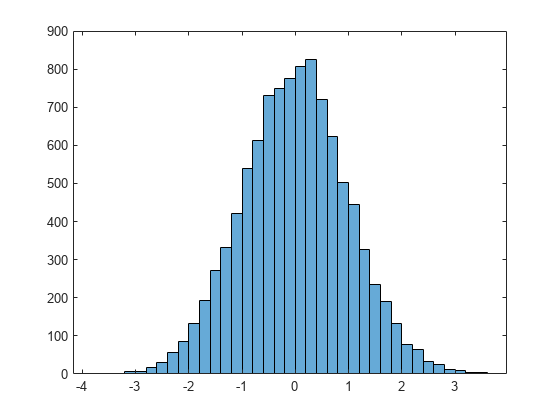
Figure contains an axes object. The axes object contains an object of type histogram.

h = Histogram with properties: Data: [10000x1 double] Values: [2 2 1 6 7 17 29 57 86 133 193 271 331 421 540 613 ... ] NumBins: 37 BinEdges: [-3.8000 -3.6000 -3.4000 -3.2000 -3 -2.8000 -2.6000 ... ] BinWidth: 0.2000 BinLimits: [-3.8000 3.6000] Normalization: 'count' FaceColor: 'auto' EdgeColor: [0 0 0] Show all properties

When you specify an output argument to thehistogramfunction, it returns a histogram object. You can use this object to inspect the properties of the histogram, such as the number of bins or the width of the bins.

Find the number of histogram bins.

nbins = h.NumBins

nbins = 37

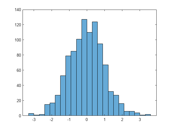
Specify Number of Histogram Bins

Open Live Script

Plot a histogram of 1,000 random numbers sorted into 25 equally spaced bins.

x = randn(1000,1); nbins = 25; h = histogram(x,nbins)

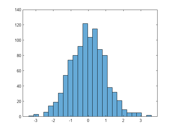
Figure contains an axes object. The axes object contains an object of type histogram.

h = Histogram with properties: Data: [1000x1 double] Values: [1 3 0 6 14 19 31 54 74 80 92 122 104 115 88 80 38 32 ... ] NumBins: 25 BinEdges: [-3.4000 -3.1200 -2.8400 -2.5600 -2.2800 -2 -1.7200 ... ] BinWidth: 0.2800 BinLimits: [-3.4000 3.6000] Normalization: 'count' FaceColor: 'auto' EdgeColor: [0 0 0] Show all properties

Find the bin counts.

counts = h.Values

counts =1×251 3 0 6 14 19 31 54 74 80 92 122 104 115 88 80 38 32 21 9 5 5 5 0 2

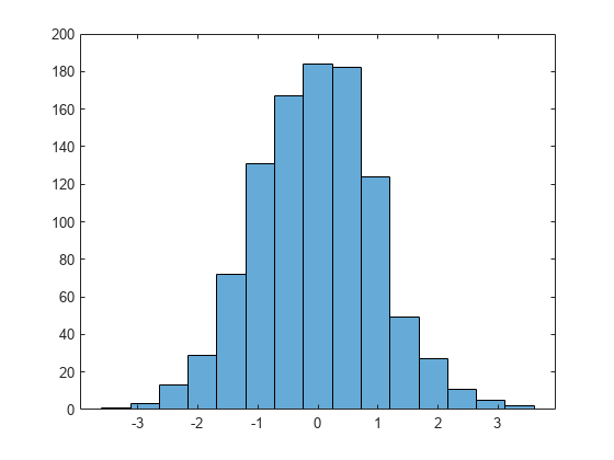
Change Number of Histogram Bins

Open Live Script

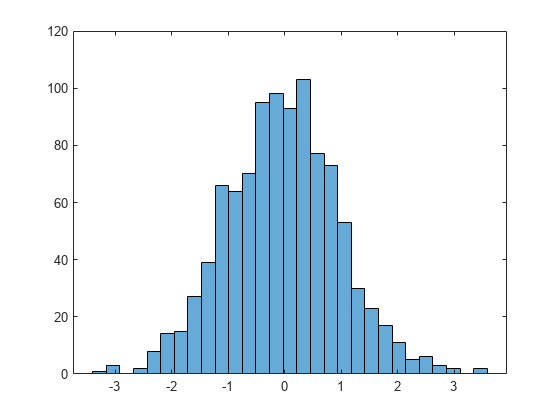
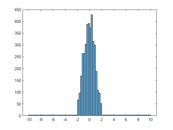
Generate 1,000 random numbers and create a histogram.

X = randn(1000,1); h = histogram(X)

Figure contains an axes object. The axes object contains an object of type histogram.

h = Histogram with properties: Data: [1000x1 double] Values: [3 1 2 15 17 27 53 79 85 101 127 110 124 95 67 32 27 ... ] NumBins: 23 BinEdges: [-3.3000 -3.0000 -2.7000 -2.4000 -2.1000 -1.8000 ... ] BinWidth: 0.3000 BinLimits: [-3.3000 3.6000] Normalization: 'count' FaceColor: 'auto' EdgeColor: [0 0 0] Show all properties

Use themorebinsfunction to coarsely adjust the number of bins.

Nbins = morebins(h); Nbins = morebins(h)

Figure contains an axes object. The axes object contains an object of type histogram.

Nbins = 29

Adjust the bins at a fine grain level by explicitly setting the number of bins.

h.NumBins = 31;

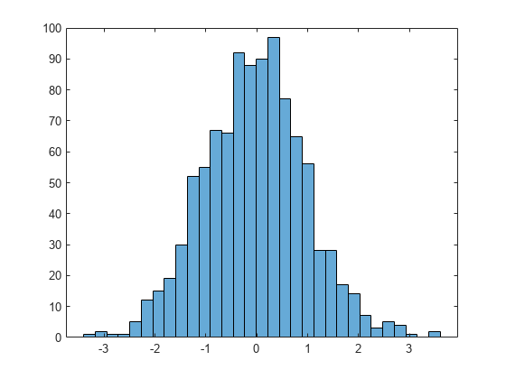
Figure contains an axes object. The axes object contains an object of type histogram.

Specify Bin Edges of Histogram

Open Live Script

Generate 1,000 random numbers and create a histogram. Specify the bin edges as a vector with wide bins on the edges of the histogram to capture the outliers that do not satisfy $| x | < 2$ . The first vector element is the left edge of the first bin, and the last vector element is the right edge of the last bin.

x = randn(1000,1); edges = [-10 -2:0.25:2 10]; h = histogram(x,edges);

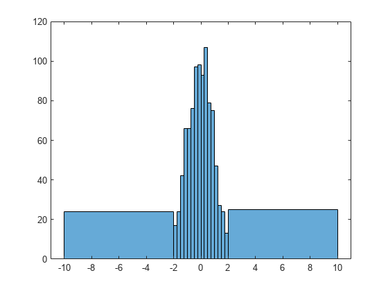
Figure contains an axes object. The axes object contains an object of type histogram.

Specify theNormalizationproperty as'countdensity'to flatten out the bins containing the outliers. Now, theareaof each bin (rather than the height) represents the frequency of observations in that interval.

h.Normalization ='countdensity';

Figure contains an axes object. The axes object contains an object of type histogram.

Plot Categorical Histogram

Open Live Script

Create a categorical vector that represents votes. The categories in the vector are'yes','no', or'undecided'.

A = [0 0 1 1 1 0 0 0 0 NaN NaN 1 0 0 0 1 0 1 0 1 0 0 0 1 1 1 1]; C = categorical(A,[1 0 NaN],{'yes','no','undecided'})

C =1x27 categoricalColumns 1 through 9 no no yes yes yes no no no no Columns 10 through 16 undecided undecided yes no no no yes Columns 17 through 25 no yes no yes no no no yes yes Columns 26 through 27 yes yes

Plot a categorical histogram of the votes, using a relative bar width of0.5.

h = histogram(C,'BarWidth',0.5)

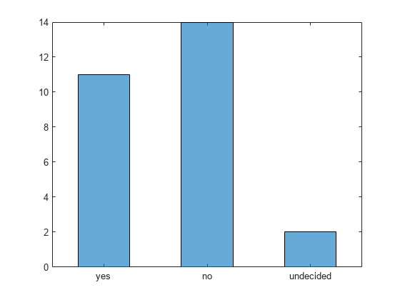
Figure contains an axes object. The axes object contains an object of type categoricalhistogram.

h = Histogram with properties: Data: [no no yes yes yes no no ... ] Values: [11 14 2] NumDisplayBins: 3 Categories: {'yes' 'no' 'undecided'} DisplayOrder: 'data' Normalization: 'count' DisplayStyle: 'bar' FaceColor: 'auto' EdgeColor: [0 0 0] Show all properties

Histogram with Specified Normalization

Open Live Script

Generate 1,000 random numbers and create a histogram using the'probability'normalization.

x = randn(1000,1); h = histogram(x,'Normalization','probability')

Figure contains an axes object. The axes object contains an object of type histogram.

h = Histogram with properties: Data: [1000x1 double] Values: [0.0030 1.0000e-03 0.0020 0.0150 0.0170 0.0270 0.0530 ... ] NumBins: 23 BinEdges: [-3.3000 -3.0000 -2.7000 -2.4000 -2.1000 -1.8000 ... ] BinWidth: 0.3000 BinLimits: [-3.3000 3.6000] Normalization: 'probability' FaceColor: 'auto' EdgeColor: [0 0 0] Show all properties

Compute the sum of the bar heights. With this normalization, the height of each bar is equal to the probability of selecting an observation within that bin interval, and the height of all of the bars sums to 1.

S = sum(h.Values)

S = 1

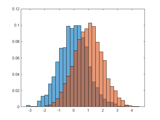
Plot Multiple Histograms

Open Live Script

Generate two vectors of random numbers and plot a histogram for each vector in the same figure.

x = randn(2000,1); y = 1 + randn(5000,1); h1 = histogram(x); holdonh2 = histogram(y);

Figure contains an axes object. The axes object contains 2 objects of type histogram.

Since the sample size and bin width of the histograms are different, it is difficult to compare them. Normalize the histograms so that all of the bar heights add to 1, and use a uniform bin width.

h1.Normalization ='probability'; h1.BinWidth = 0.25; h2.Normalization ='probability'; h2.BinWidth = 0.25;

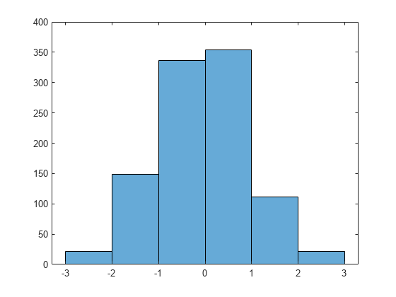
Figure contains an axes object. The axes object contains 2 objects of type histogram.

Adjust Histogram Properties

Open Live Script

Generate 1,000 random numbers and create a histogram. Return the histogram object to adjust the properties of the histogram without recreating the entire plot.

x = randn(1000,1); h = histogram(x)

Figure contains an axes object. The axes object contains an object of type histogram.

h = Histogram with properties: Data: [1000x1 double] Values: [3 1 2 15 17 27 53 79 85 101 127 110 124 95 67 32 27 ... ] NumBins: 23 BinEdges: [-3.3000 -3.0000 -2.7000 -2.4000 -2.1000 -1.8000 ... ] BinWidth: 0.3000 BinLimits: [-3.3000 3.6000] Normalization: 'count' FaceColor: 'auto' EdgeColor: [0 0 0] Show all properties

Specify exactly how many bins to use.

h.NumBins = 15;

Figure contains an axes object. The axes object contains an object of type histogram.

Specify the edges of the bins with a vector. The first value in the vector is the left edge of the first bin. The last value is the right edge of the last bin.

h.BinEdges = [-3:3];

Figure contains an axes object. The axes object contains an object of type histogram.

Change the color of the histogram bars.

h.FaceColor = [0 0.5 0.5]; h.EdgeColor ='r';

Figure contains an axes object. The axes object contains an object of type histogram.

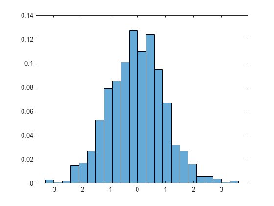
Determine Underlying Probability Distribution

Open Live Script

Generate 5,000 normally distributed random numbers with a mean of 5 and a standard deviation of 2. Plot a histogram withNormalizationset to'pdf'to produce an estimation of the probability density function.

x = 2*randn(5000,1) + 5; histogram(x,'Normalization','pdf')

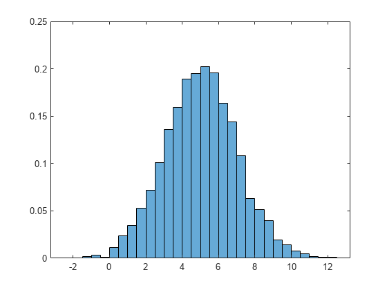
Figure contains an axes object. The axes object contains an object of type histogram.

In this example, the underlying distribution for the normally distributed data is known. You can, however, use the'pdf'histogram plot to determine the underlying probability distribution of the data by comparing it against a known probability density function.

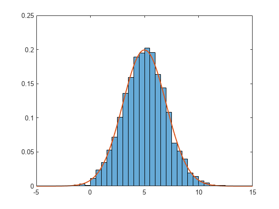
The probability density function for a normal distribution with mean $μ$ , standard deviation $σ$ , and variance $σ^{2}$ is

$f (x, μ, σ) = \frac{1}{σ \sqrt{2 π}} exp [- \frac{(x - μ)^{2}}{2 σ^{2}}] .$

Overlay a plot of the probability density function for a normal distribution with a mean of 5 and a standard deviation of 2.

holdony = -5:0.1:15; mu = 5; sigma = 2; f = exp(-(y-mu).^2./(2*sigma^2))./(sigma*sqrt(2*pi)); plot(y,f,'LineWidth',1.5)

Figure contains an axes object. The axes object contains 2 objects of type histogram, line.

Saving and Loading Histogram Objects

Open Live Script

Use thesavefigfunction to save ahistogramfigure.

histogram(randn(10)); savefig('histogram.fig'); closegcf

Useopenfigto load the histogram figure back into MATLAB.openfigalso returns a handle to the figure,h.

h = openfig('histogram.fig');

Figure contains an axes object. The axes object contains an object of type histogram.

Use thefindobjfunction to locate the correct object handle from the figure handle. This allows you to continue manipulating the original histogram object used to generate the figure.

y = findobj(h,'type','histogram')

y = Histogram with properties: Data: [10x10 double] Values: [2 17 28 32 16 3 2] NumBins: 7 BinEdges: [-3 -2 -1 0 1 2 3 4] BinWidth: 1 BinLimits: [-3 4] Normalization: 'count' FaceColor: 'auto' EdgeColor: [0 0 0] Show all properties

Tips

Histogram plots created usinghistogramhave a context menu in plot edit mode that enables interactive manipulations in the figure window. For example, you can use the context menu to interactively change the number of bins, align multiple histograms, or change the display order.
When you add data tips to a histogram plot, they display the bin edges and bin count.

Extended Capabilities

Tall Arrays
Calculate with arrays that have more rows than fit in memory.

This function supports tall arrays with the limitations:

Some input options are not supported. The allowed options are:
- 'BinWidth'
- 'BinLimits'
- 'Normalization'
- 'DisplayStyle'
- 'BinMethod'— The'auto'and'scott'bin methods are the same. The'fd'bin method is not supported.
- 'EdgeAlpha'
- 'EdgeColor'
- 'FaceAlpha'
- 'FaceColor'
- 'LineStyle'
- 'LineWidth'
- 'Orientation'
Additionally, there is a cap on the maximum number of bars. The default maximum is 100.
Themorebinsandfewerbinsmethods are not supported.
Editing properties of the histogram object that require recomputing the bins is not supported.

For more information, seeTall Arrays for Out-of-Memory Data.

GPU数组
Accelerate code by running on a graphics processing unit (GPU) using Parallel Computing Toolbox™.

Usage notes and limitations:

This function accepts GPU arrays, but does not run on a GPU.

For more information, seeRun MATLAB Functions on a GPU(Parallel Computing Toolbox).

Distributed Arrays
Partition large arrays across the combined memory of your cluster using Parallel Computing Toolbox™.

Usage notes and limitations:

This function operates on distributed arrays, but executes in the client MATLAB.

For more information, seeRun MATLAB Functions with Distributed Arrays(Parallel Computing Toolbox).

Version History

Introduced in R2014b

histogram

Description

Creation

Syntax

Description

Input Arguments

X—数据分发垃圾箱中vector|matrix|multidimensional array

C—Categorical datacategorical array

nbins—Number of binspositive integer

edges—Bin edgesvector

Categories—Categories included in histogramcell array of character vectors|categorical array|string array

counts—Bin countsvector

ax—Target axesAxesobject|PolarAxesobject

BarWidth—Relative width of categorical bars0.9(default) |scalar in range[0,1]

BinLimits—Bin limitstwo-element vector

BinLimitsMode—Selection mode for bin limits'auto'(default) |'manual'

BinMethod—Binning algorithm'auto'(default) |'scott'|'fd'|'integers'|'sturges'|'sqrt'| ...

BinWidth—Width of binsscalar

DisplayOrder—Category display order'data'(default) |'ascend'|'descend'

DisplayStyle—Histogram display style'bar'(default) |'stairs'

EdgeAlpha—Transparency of histogram bar edges1(default) |scalar value between0and1inclusive

EdgeColor—Histogram edge color[0 0 0]或黑色(default) |'none'|'auto'|RGB triplet|hexadecimal color code|color name

FaceAlpha—Transparency of histogram bars0.6(default) |scalar value between0and1inclusive

FaceColor—Histogram bar color'auto'(default) |'none'|RGB triplet|hexadecimal color code|color name

LineStyle—Line style“- - -”(default) |'--'|':'|'-.'|'none'

LineWidth—Width of bar outlines0.5(default) |positive value

Normalization—Type of normalization'count'(default) |'probability'|'countdensity'|'pdf'|'cumcount'|'cdf'

NumDisplayBins—Number of categories to displayscalar

Orientation—Orientation of bars'vertical'(default) |'horizontal'

ShowOthers—Toggle summary display of data belonging to undisplayed categories'off'(default) |on/off logical value

Output Arguments

h— Histogramobject

Properties

Object Functions

Examples

Histogram of Vector

Specify Number of Histogram Bins

Change Number of Histogram Bins

Specify Bin Edges of Histogram

Plot Categorical Histogram

Histogram with Specified Normalization

Plot Multiple Histograms

Adjust Histogram Properties

Determine Underlying Probability Distribution

Saving and Loading Histogram Objects

Tips

Extended Capabilities

Tall ArraysCalculate with arrays that have more rows than fit in memory.

GPU数组Accelerate code by running on a graphics processing unit (GPU) using Parallel Computing Toolbox™.

Distributed ArraysPartition large arrays across the combined memory of your cluster using Parallel Computing Toolbox™.

Version History

See Also

Topics

`X`—数据分发垃圾箱中
vector|matrix|multidimensional array

`C`—Categorical data
categorical array

`nbins`—Number of bins
positive integer

`edges`—Bin edges
vector

`Categories`—Categories included in histogram
cell array of character vectors|categorical array|string array

`counts`—Bin counts
vector

`ax`—Target axes
`Axes`object|`PolarAxes`object

`BarWidth`—Relative width of categorical bars
`0.9`(default) |scalar in range`[0,1]`

`BinLimits`—Bin limits
two-element vector

`BinLimitsMode`—Selection mode for bin limits
`'auto'`(default) |`'manual'`

`BinMethod`—Binning algorithm
`'auto'`(default) |`'scott'`|`'fd'`|`'integers'`|`'sturges'`|`'sqrt'`| ...

`BinWidth`—Width of bins
scalar

`DisplayOrder`—Category display order
`'data'`(default) |`'ascend'`|`'descend'`

`DisplayStyle`—Histogram display style
`'bar'`(default) |`'stairs'`

`EdgeAlpha`—Transparency of histogram bar edges
`1`(default) |scalar value between`0`and`1`inclusive

`EdgeColor`—Histogram edge color
`[0 0 0]`或黑色(default) |`'none'`|`'auto'`|RGB triplet|hexadecimal color code|color name

`FaceAlpha`—Transparency of histogram bars
`0.6`(default) |scalar value between`0`and`1`inclusive

`FaceColor`—Histogram bar color
`'auto'`(default) |`'none'`|RGB triplet|hexadecimal color code|color name

`LineStyle`—Line style
`“- - -”`(default) |`'--'`|`':'`|`'-.'`|`'none'`

`LineWidth`—Width of bar outlines
`0.5`(default) |positive value

`Normalization`—Type of normalization
`'count'`(default) |`'probability'`|`'countdensity'`|`'pdf'`|`'cumcount'`|`'cdf'`

`NumDisplayBins`—Number of categories to display
scalar

`Orientation`—Orientation of bars
`'vertical'`(default) |`'horizontal'`

`ShowOthers`—Toggle summary display of data belonging to undisplayed categories
`'off'`(default) |on/off logical value

`h`— Histogram
object

Tall Arrays
Calculate with arrays that have more rows than fit in memory.

GPU数组
Accelerate code by running on a graphics processing unit (GPU) using Parallel Computing Toolbox™.

Distributed Arrays
Partition large arrays across the combined memory of your cluster using Parallel Computing Toolbox™.